Analyzing Metadata from Spotify Playlists

Download Metadata

The original blog post lays out the steps you need to install everything properly, so I won’t repeat them here. However, I’ll briefly go over a few problems I encountered while trying to get it to work in the context of RStudio.

1. The blog post tells you to run pip install -r requirements.txt to install the necessary packages for their GSA module. If you are using reticulate in R/RStudio 1.4, you may also need to install those packages with py_install so that those packages are installing to the environment used by reticulate.

2. In order for import GSA to work, Python has to be able to find GSA.py (and the other python scripts) in either the current working directory or some other directory that Python knows to search in. You can check what the current working directory is with os.getcwd(). If it is not there, then you can add the directory containing GSA.py to the path with sys.path.insert. For example, in my case, when I downloaded the Python scripts, I had them in a subdirectory of my project folder, so I had to add that subdirectory, “GeneralizedSpotifyAnalyser-main,” to my Python path:

import os
os.getcwd() # Check where you working directory is
import sys
sys.path.insert(0, './GeneralizedSpotifyAnalyser-main') # Add subdirectory to path
import GSA
import pandas as pd

After successfully importing GSA, I followed the sample script GSA_basicExample.py to download the playlist metadata. The playlist I’m using as an example is “Chillin’ on a Dirt Road.”

GSA.authenticate()
# Here's an example playlist ID: 37i9dQZF1DX3hgbB9nrEB1
myPlaylist = GSA.getInformation('37i9dQZF1DX3hgbB9nrEB1', verbose=True)
# Read the .pkl-file to get a dataframe
myPlaylistInformation = pd.read_pickle(myPlaylist)

I also modified the GSA.getInformation function slightly to add an additional column for artist names. If you poke around the track variable in the function, you may also find other metadata fields that you are interested in, since the function by default doesn’t save all of the fields into the data frame. The artists are under track['track']['artists'] and their names can be accessed in Python as [x['name'] for x in track['track']['artists']].

Regarding RStudio 1.4’s integration with Python, I did have quite a smooth experience running everything. I could send lines of Python code to the RStudio console just like R code. I also noticed that RStudio will automatically detect whether you are trying to run Python or R code and enter and exit reticulate for you. In addition, Python variables show up in the Environment tab of RStudio, which isn’t something I personally use a lot, but it’s still cool to see. Based on this limited experience, RStudio seems to be able to function like an IDE for Python.

Some of these features may have already existed pre-RStudio 1.4, because I will say that the last time I used reticulate, I remember having a rather good experience already. For example, something really cool about reticulate is that you can switch from Python back to R and access any Python object with py$name_of_object. I don’t know how this extraordinary magic is implemented, but it’s amazing.

playlist_meta_raw = py$myPlaylistInformation

Below I’ve print out the data frame in R, which was originally downloaded in Python.

head(playlist_meta_raw)

## # A tibble: 6 x 21
##      X1 playlistID  TrackName  TrackID  SampleURL   ReleaseYear Artists Genres  
##   <dbl> <chr>       <chr>      <chr>    <chr>       <chr>       <chr>   <chr>   
## 1     0 37i9dQZF1D… Worth It   5APWbHd… https://p.… 2017-12-01  ['Dani… ['alt z…
## 2     1 37i9dQZF1D… Seeing Bl… 65wnZsZ… https://p.… 2017-10-20  ['Nial… ['dance…
## 3     2 37i9dQZF1D… I Could U… 09iyGil… https://p.… 2017-03-17  ['Mare… ['conte…
## 4     3 37i9dQZF1D… I Want Cr… 4FkgULe… https://p.… 2011        ['Hunt… ['conte…
## 5     4 37i9dQZF1D… Downtown   4kY7rYt… https://p.… 2013-01-01  ['Lady… ['conte…
## 6     5 37i9dQZF1D… Tequila    7Il2yWQ… https://p.… 2018-01-10  ['Dan … ['conte…
## # … with 13 more variables: danceability <dbl>, energy <dbl>, loudness <dbl>,
## #   speechiness <dbl>, acousticness <dbl>, instrumentalness <dbl>,
## #   liveness <dbl>, valence <dbl>, tempo <dbl>, key <dbl>, mode <dbl>,
## #   duration_ms <dbl>, Popularity <dbl>

Plot the Data

Once I have the data, I can make all sorts of interesting plots. First, I clean up the data a bit using the R packages janitor (for column names) and lubridate (for dates).

playlist_meta = playlist_meta_raw %>%
  as_tibble() %>%
  clean_names()

playlist_meta = playlist_meta %>%
  mutate(release_date = ymd(release_year, truncated = 2),
         release_year = year(release_date)) 

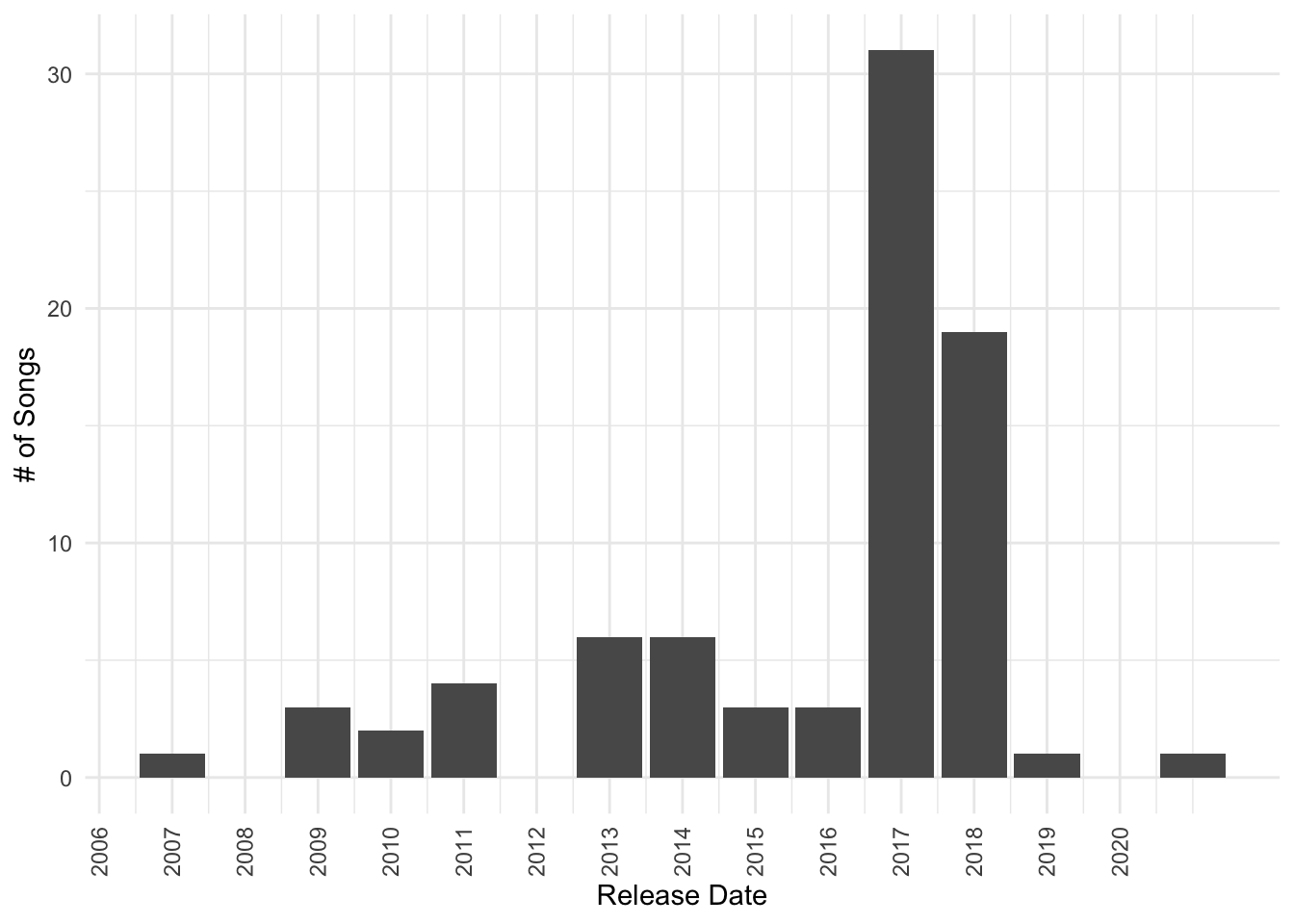
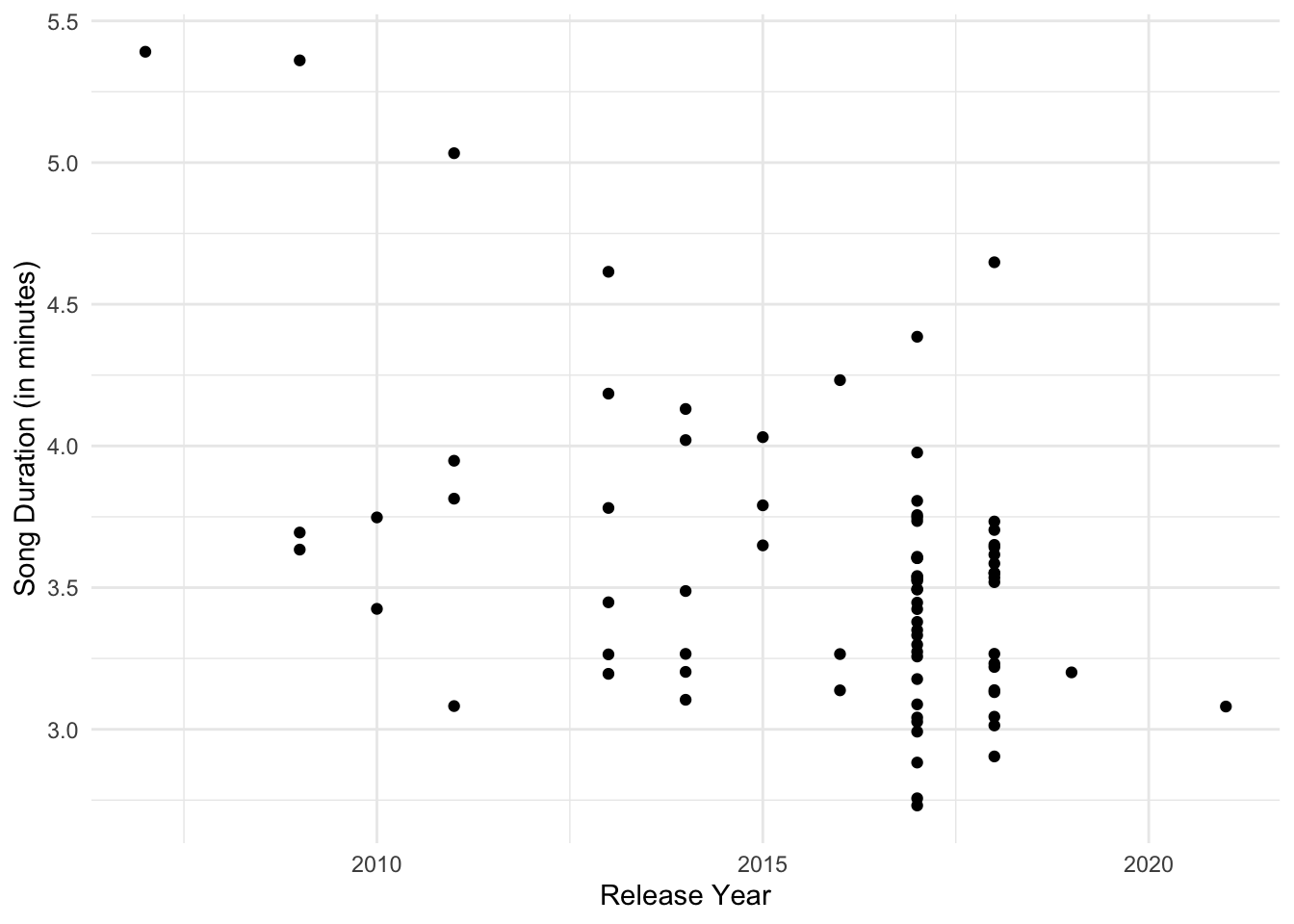
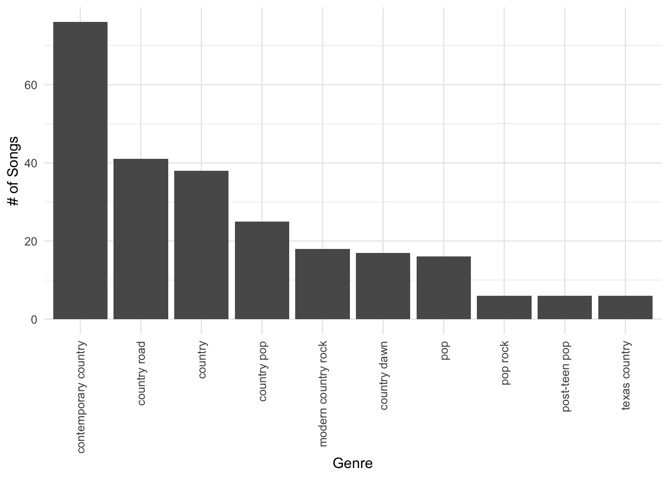
Then I use ggplot2 to make some fun visualizations of the songs in the playlist.

# Release date
playlist_meta %>%
  ggplot(aes(x = release_year)) +
  geom_bar() +
  scale_x_continuous(breaks = 1990:2020) +
  labs(x = "Release Date",
       y = "# of Songs") +
  theme_minimal() +
  theme(axis.text.x = element_text(angle = 90, vjust = 0.5, hjust=1))

# Song duration
playlist_meta %>%
  ggplot(aes(x = release_year, y = duration_ms/1000/60)) +
  geom_point() +
  labs(x = "Release Year",
       y = "Song Duration (in minutes)") +
  theme_minimal()

# Genres
# Table of counts for genres (each song counted multiple times)
popular_genres = sapply(playlist_meta$genres, function(x) strsplit(gsub("(\\[)|(\\])|(\\')","",x), ", ")) %>%
  unname() %>%
  unlist() %>%
  table()
popular_genres_tb = tibble(genres = names(popular_genres),
                           count = popular_genres) %>%
  arrange(-count)

popular_genres_tb %>%
  uncount(as.integer(count)) %>%
  mutate(genres = fct_lump_n(fct_infreq(genres), 10)) %>%
  filter(genres != "Other") %>%
  ggplot(aes(x = genres)) +
  geom_bar() +
  labs(x = "Genre", y = "# of Songs") +
  theme_minimal() +
  theme(axis.text.x = element_text(angle = 90, vjust = 0.5, hjust=1))